Generative Adversarial Networks

A Generative Adversarial Network (GAN) is a powerful method for generating samples from an unknown distribution, particularly hard to model distributions such as images. In this post we will shortly introduce the GAN model, and then focus on two major failure modes of these models, namely Vanishing Gradient and Mode Collapse. We will conclude by briefly mentioning the state of the art methods in GAN literature. Note that this post is mainly focused on certain theoretical analysis of the failure modes of GANs, for details of algorithms and their respective guarantees see the referenced papers.

1. Definitions

We start by looking at the task definition and the way GANs try to model the task.

1.1. Problem Statement

Let ${p(x): {\cal X} \rightarrow (0,1)}$ be the real data distribution and ${g(x; \theta): {\cal X} \rightarrow (0,1)}$ be the model distribution parametrized by ${\theta}$ . Given m samples from ${p(x)}$ the task is to estimate ${g(x;\theta)}$ “close” to ${p(x)}$ . We may refer to ${\cal X}$ as image space in the remainder of this post, however it can be any data distribution. Notice that there are many ways to model this task, for example the kernel density estimation methods model ${g(x)}$ by windows passing over the given samples. Next we will look at the adversarial modeling of this task by [Goodfellow et al. 2014].

1.2. GAN Model

Consider the following continuous differentiable functions (e.g. defined by Neural Nets):

$\displaystyle G(z;\theta): {\mathbb R}^h \rightarrow {\cal X}$

$\displaystyle D(x;w): {\cal X} \rightarrow [0, 1]$

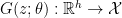
We refer to ${G}$ as the “generator” and ${g(x;\theta)}$ is the model distribution induced by sampling from this function using ${z \sim U(-1,1)^h}$ . We refer to ${D}$ as the “discriminator” and it is essentially a binary classifier (before thresholding). We might drop the parameters ${\theta}$ and ${w}$ for brevity in some equations. We further assume that ${G}$ and ${D}$ are universal approximators.

The idea is to train ${D}$ towards perfectly discriminating real samples ${x \sim p(x)}$ from fake samples ${x \sim g(x)}$ , and in turn train ${G}$ towards confusing ${D}$ , hence the term “Adversarial Networks”, and in doing so we conjecture that ${G}$ would end up generating samples “close” to the real data distribution. More concretely we define a loss as follows:

$\displaystyle L(\theta, w) = \mathop{\mathbb E}_{x \sim p} \log D(x) + \mathop{\mathbb E}_{x \sim g} \log (1-D(x)) \ \ \ \ \ (1)$

Or equivalently:

$\displaystyle L(\theta, w) = \mathop{\mathbb E}_{x \sim p} \log D(x) + \mathop{\mathbb E}_{z \sim U} \log (1-D(G(z))$

And then the training process is:

$\displaystyle G^* = {arg\min}_{\theta} {\max}_{w} L(\theta, w) \ \ \ \ \ (2)$

Note that we use ${G^*}$ and ${\theta^*}$ interchangeably to refer to optimal generator, similarly for discriminator. This optimization is formulated to capture the mentioned adversarial intuition, however this is of course not the only way to model the intuition, a point to which we’ll return at the end of this blog post.

2. Theorems and Analysis

In this section we first provide a theoretical validation for the GAN model, and then provide theorems and analysis regarding the failure modes of GANs.

2.1. GAN Convergence

The optimization defined in Equation (2) intuitively brings ${g(x)}$ close to ${p(x)}$ , however we need a more concrete guarantee that this in fact happens. The following theorem by [Goodfellow et al. 2014] shows that at the optimum, the solution to Equation (2) is ${g(x) = p(x)}$ .

Theorem 1 The result of ${G^* = {arg\min}_{\theta} {\max}_{w} L(\theta, w)}$ is ${g(x;\theta^*) = p(x)}$ .

Proof: We first rewrite ${L(\theta,w)}$ in its integral form:

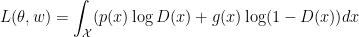
$\displaystyle L(\theta, w) = \int_{\cal X} ( p(x) \log D(x) + g(x) \log (1-D(x)) dx$

Now at each ${x}$ , we find ${D(x)}$ that maximizes the term inside the integral, by taking the derivative wrt ${D(x)}$ :

$\displaystyle \frac {p(x)} {D(x)} - \frac {g(x)} {1-D(x)} = 0$

$\displaystyle D(x) = \frac {p(x)} {p(x)+g(x)}$

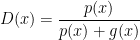
Thus we have:

$\displaystyle D^* = arg\max_{w} L(\theta,w) = \frac {p(x)} {p(x)+g(x)}$

Now we replace this ${D^*}$ into the definition of ${L(\theta, w)}$ :

$\displaystyle L(\theta, w^*) = \max_{w} L(\theta,w) = \mathop{\mathbb E}_{x \sim p} \log \frac {p(x)} {p(x)+g(x)} + \mathop{\mathbb E}_{x \sim g} \log \frac {g(x)} {p(x)+g(x)}$

Given the definition of Kullback Leibler Divergence ${KL(p||g) = \mathop{\mathbb E}_{x \sim p} \log \frac {p(x)} {p(x)+g(x)}}$ we have:

$\displaystyle L(\theta, w^*) = KL(p||\frac {p+g} 2) + KL(g||\frac {p+g} 2) - 2\log 2$

$\displaystyle L(\theta, w^*) = 2JSD(p||g) - 2\log 2$

where ${JSD(p||g)}$ is the Jensen Shannon Divergence and is replaced by definition. It is known that ${0 \leq JSD(p||g) \leq 2\log2}$ , and the lower bound equality only happens when ${p=g}$ . Thus the result of ${G^* = {arg\min}_{\theta} L(\theta, w^*) = {arg\min}_{\theta} 2JSD(p||g)}$ is ${g(x;\theta) = p(x)}$ over ${\cal X}$ . $\Box$

2.2. Vanishing Gradient

Before we provide a theorem describing the Vanishing Gradient issue, we need to consider some assumptions and their implications on the support of ${p(x)}$ and ${g(x)}$ . We will only briefly discuss the next two theorems to provide a basis for analyzing vanishing gradient, look at [Arjovsky and Bottou, 2017] for the proofs.

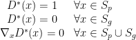
Theorem 2 Let ${S_p \in \cal X}$ and ${S_g \in \cal X}$ be the supports of ${p(x)}$ and ${g(x)}$ respectively. Assume ${S_p}$ and ${S_g}$ are disjoint compact sets, then there exists a smooth continuous function ${D^*: {\cal X} \rightarrow [0,1]}$ such that:

$\displaystyle \begin{array}{rcl} &D^*(x) = 1 &\forall x \in S_p \\ &D^*(x) = 0 &\forall x \in S_g \\ &\nabla_x D^*(x) = 0 &\forall x \in S_p \cup S_g \end{array}$

The next theorem extends Theorem 2 to the case where the supports are manifolds rather than sets.

Theorem 3 Let ${S_p \in \cal X}$ and ${S_g \in \cal X}$ be the supports of ${p(x)}$ and ${g(x)}$ respectively. Assume ${S_p}$ and ${S_g}$ are manifolds that are not full dimension and not perfectly aligned, then there exists a smooth continuous function ${D^*: {\cal X} \rightarrow [0,1]}$ such that:

$\displaystyle \begin{array}{rcl} &D^*(x) = 1 &\forall x \in S_p \\ &D^*(x) = 0 &\forall x \in S_g \\ &\nabla_x D^*(x) = 0 &\forall x \in S_p \cup S_g \end{array}$

To see what Theorem 3 means assume ${\cal X}$ is the 2D plane. Then if real data and fake data come from two closed 1D shapes that only intersect in a finite number of points (e.g. two unit circles centered at (0.5, 0) and (-0.5, 0)) then Theorem 3 tells us that there exists a binary classifier that can perfectly separate them and be completely flat over each manifold. The assumptions are often valid in the real world tasks, specifically when considering the manifold of real images and the manifold of generated images by ${G(z)}$ if ${dim(z) < dim({\cal X})}$ .

Now we are ready to investigate the problem of vanishing gradient. The optimization in Equation (2) suggests we should train ${D}$ till convergence and then take a step towards training ${G}$ , and repeat this process. However the following theorem by [Arjovsky and Bottou, 2017] shows that training ${D}$ till convergence results in loss of the gradient signal for updating ${G}$ and therefore hinders the optimization task.

Theorem 4 Given assumptions of Theorem 3 or 2, and assuming ${||D-D^*|| < \epsilon}$ and ${\mathop{\mathbb E}_{z\sim U} ||J_{\theta} G(z)||_2^2 \leq M^2}$ , then:

$\displaystyle || \mathop{\mathbb E}_{z\sim U} \nabla_{\theta} \log (1-D(G(z)))||_2 \leq M \frac {\epsilon}{1-\epsilon}$

where ${||D||}$ is defined as follows:

$\displaystyle ||D|| = \sup_{x} |D(x)| + ||\nabla_x D(x)||_2$

Before we prove this theorem let’s look at an immediate corollary of this theorem:

Corollary 5 Given assumptions of Theorem 4:

$\displaystyle \lim_{||D-D^*|| \rightarrow 0} || \mathop{\mathbb E}_{z\sim U} \nabla_{\theta} \log (1-D(G(z)))||_2 = 0$

Therefore this corollary shows that if we find the optimal ${D}$ and replace it in ${L(\theta,w)}$ , the gradient wrt ${\theta}$ would be zero, hence the term Vanishing Gradient. Now let’s look at the proof for Theorem 4.

Proof: We start by the squared of the left hand side. Since norm 2 is a convex function, we can use Jensen’s inequality to bring the expectation out of the norm, and then apply chain rule:

$\displaystyle || \mathop{\mathbb E}_{z\sim U} \nabla_{\theta} \log (1-D(G(z)))||_2^2 \leq \mathop{\mathbb E}_{z\sim U} \frac {||J_{\theta} G(z) \nabla_{x} D(G(z))||_2^2} {|1 - D(G(z))|^2}$

where ${J_{\theta}}$ is the Jacobian wrt ${\theta}$ . Now note that ${J \nabla}$ is projecting the gradient vector ${\nabla}$ using matrix ${J}$ , and by definition the maximum factor by which a projection can increase the norm of a vector is the largest singular value of the projection matrix, known as the spectral norm of a matrix denoted by ${||J||_2}$ . Therefore we have:

$\displaystyle \mathop{\mathbb E}_{z\sim U} \frac {||J_{\theta} G(z) \nabla_{x} D(G(z))||_2^2} {|1 - D(G(z))|^2} \leq \mathop{\mathbb E}_{z\sim U} \frac {||J_{\theta} G(z)||_2^2 ||\nabla_{x} D(G(z))||_2^2} {|1 - D(G(z))|^2}$

Using the definition of ${||D||}$ on the assumption ${||D-D^*|| < \epsilon}$ we can write:

$\displaystyle ||D-D^*|| = \sup_{x} |D(x)-D^*(x)| + ||\nabla_x D(x) - \nabla_x D^*(x)||_2 < \epsilon$

Therefore for all ${x \in \cal X}$ we have ${D(x)-D^*(x) < \epsilon}$ and ${||\nabla_x D(x)||_2 - ||\nabla_x D^*(x)||_2 < \epsilon}$ . Using these inequalities we have:

$\displaystyle \mathop{\mathbb E}_{z\sim U} \frac {||J_{\theta} G(z)||_2^2 ||\nabla_{x} D(G(z))||_2^2} {|1 - D(G(z))|^2} < \mathop{\mathbb E}_{z\sim U} \frac {||J_{\theta} G(z)||_2^2 (||\nabla_{x} D^*(G(z))||_2 + \epsilon)^2} {(|1 - D^*(G(z))| - \epsilon)^2}$

Now note that by Theorem 3 or 2, we know that ${\nabla_{x} D^*(x) = 0}$ and ${D^*(x) = 0}$ for all ${x \in S_g}$ , thus:

$\displaystyle = \mathop{\mathbb E}_{z\sim U} \frac {||J_{\theta} G(z)||_2^2 (\epsilon)^2} {(1 - \epsilon)^2} \leq M^2 \frac {\epsilon^2}{(1-\epsilon)^2}$

Taking a square root finishes the proof. $\Box$

2.3. Modified GAN and Mode Collapse

In order to avoid the vanishing gradient issue, [Goodfellow et al. 2014] suggests a modified update rule for the generator as follows:

$\displaystyle \Delta \theta = \mathop{\mathbb E}_{z\sim U} -\nabla_{\theta} log D(G(z))$

However the following theorem by [Arjovsky and Bottou, 2017] reveals an important flaw in this modified formulation:

Theorem 6 Let ${D^* = \frac {p(x)}{g(x; \theta_0) + p(x)}}$ be the optimal discriminator at ${\theta_0}$ . Then:

$\displaystyle \mathop{\mathbb E}_{z\sim U} -\nabla_{\theta} log D^*(G(z)) |_{\theta={\theta}_0} = \nabla_{\theta}[ KL(g||p) - 2JSD(p || g)]|_{\theta={\theta}_0}$

Before we provide the proof, let’s analyze what this theorem means. It shows that minimizing the modified objective results in minimizing KL(g||p) and maximizing JSD(p||g). The latter tries to push the distributions apart. On the other hand KL greatly penalizes high probability regions in g that have low probability in p, however does not penalizes the reverse as much. That means KL(g||p) does not penalizes much collapsing the density of g on a single mode of p. Therefore the optimum of maximizing reverse KL and JSD between two distribution happens exactly when g collapses all its density on a single mode of p, resulting in high JSD and low KL. Next we’ll prove Theorem 6.

Proof: We start by writing the definition of KL(g||p) as follows:

$\displaystyle KL(g||p) = \mathop{\mathbb E}_{x\sim g} \log \frac gp = \mathop{\mathbb E}_{x\sim g} \log \frac {g(x;{\theta}_0)}{p} + \mathop{\mathbb E}_{x\sim g} \log \frac {g}{g(x;{\theta}_0)}$

Now replacing the definition of ${D^*}$ we get:

$\displaystyle = \mathop{\mathbb E}_{x\sim g} \log \frac {1-D^*}{D^*} + \mathop{\mathbb E}_{x\sim g} \log \frac {g}{g(x;{\theta}_0)} = - \mathop{\mathbb E}_{z\sim U} \log \frac {D^*(G(z))}{1-D^*(G(z))} + KL(g || g(x;{\theta}_0))$

Next we take a gradient wrt ${\theta}$ at ${\theta_0}$ . Note that the gradient of ${KL(g(x) || g(x;{\theta}_0))}$ is zero at ${\theta_0}$ since the distributions are the same. Therefore we have:

$\displaystyle \nabla_\theta KL(g||p)|_{\theta=\theta_0} = \mathop{\mathbb E}_{z \sim U} -\nabla_\theta \log \frac {D^*(G(z))}{1-D^*(G(z))}|_{\theta=\theta_0}$

Finally note that from Theorem 1 we have:

$\displaystyle \mathop{\mathbb E}_{z \sim U} \nabla_\theta \log (1-D^*(G(z)))|_{\theta=\theta_0} = \nabla_\theta 2JSD(p||g)|_{\theta=\theta_0}$

Calculating ${\nabla_\theta KL(g||p)|_{\theta=\theta_0} - \nabla_\theta 2JSD(p||g)|_{\theta=\theta_0}}$ completes the proof. $\Box$

2.4. A Simple Solution

To solve the problem of Vanishing Gradient, we can simply add noise to both the output of generator and the real data. Doing so will increase the overlap between ${S_p}$ and ${S_g}$ . Therefore it violates the assumptions of Theorem 3 and 2 and thus no longer necessarily faces Vanishing Gradient. See [Arjovsky and Bottou, 2017] for details of this noisy version of GAN and some nice properties.

2.5. A Grain of Salt

An important point to note is that the results of Theorems 1 and 6 are based on assuming the behavior of optimal discriminator. However, when optimizing ${D}$ , the loss does not necessarily becomes a better estimate of the divergence, the divergence only occurs at optimal ${D}$ . This means that minimizing generator loss does not necessarily minimize the divergence at each step. See [Fedus et al. 2017] for more details on this point.

3. State of the Art

In this section we briefly introduce Wasserstein GAN formulation and mention some very recent works focused on the problem of Mode Collapse.

3.1. Wasserstein GAN

Wasserstein GAN [Arjovsky et al. 2017] uses the following formulation:

$\displaystyle G(z;\theta): {\mathbb R}^h \rightarrow {\cal X}$

$\displaystyle D(x;w): {\cal X} \rightarrow {\mathbb R}$

$\displaystyle L(\theta, w) = \mathop{\mathbb E}_{x \sim p} D(x) - \mathop{\mathbb E}_{z \sim U} D(G(z))$

$\displaystyle G^* = {arg\min}_{\theta} {\max}_{w} L(\theta, w)$

Where ${D}$ is a 1-Lipschitz function. Notice that the main difference is using a real valued ${D}$ , called the “critic” instead of discriminator, and removing the log in ${L(\theta, w)}$ . Here ${{\max}_{w} L(\theta, w)}$ is actually approximating the dual of wasserstein distance between ${p(x)}$ and ${g(x)}$ , and then the generator tries to minimize this distance. The advantage is that wasserstein distance is sensitive to sample locations and not just their density, but more importantly here optimizing ${D}$ explicitly improves the estimate of wasserstein distance, whereas in regular GAN optimizing discriminator does not improve the estimate to JSD explicitly.

3.2. More recent works

Unrolled GAN [Metz et al. 2016], VEE-GAN [Srivastava et al. 2017] and Bi-GAN [Donahue et al. 2016] are recent approaches also addressing the problem of mode collapse.

References

Goodfellow, Ian, et al. “Generative adversarial nets.” Advances in neural information processing systems. 2014.

Arjovsky, Martin, and Léon Bottou. “Towards principled methods for training generative adversarial networks.” arXiv preprint arXiv:1701.04862 (2017).

Fedus, William, et al. “Many Paths to Equilibrium: GANs Do Not Need to Decrease aDivergence At Every Step.” arXiv preprint arXiv:1710.08446 (2017).

Metz, Luke, et al. “Unrolled generative adversarial networks.” arXiv preprint arXiv:1611.02163 (2016).

Srivastava, Akash, et al. “VEEGAN: Reducing Mode Collapse in GANs using Implicit Variational Learning.” arXiv preprint arXiv:1705.07761 (2017).

Donahue, Jeff, Philipp Krähenbühl, and Trevor Darrell. “Adversarial feature learning.” arXiv preprint arXiv:1605.09782 (2016).

Arjovsky, Martin, Soumith Chintala, and Léon Bottou. “Wasserstein gan.” arXiv preprint arXiv:1701.07875 (2017).